P-value | Strength of evidence |
|---|---|
<0.001 | Very strong evidence |
0.001 to <0.01 | Strong evidence |
0.01 to <0.05 | Evidence |
0.05 to <0.1 | Weak evidence |
≥0.1 | Little or no evidence |
Learning objectives
By the end of this module you will be able to:
- Formulate a research question as a hypothesis;
- Understand the concepts of a hypothesis test;
- Consider the difference between statistical significance and clinical importance;
- Use 95% confidence intervals to conduct an informal hypothesis test;
- Perform and interpret a one-sample t-test;
- Explain the concept of one and two tailed statistical tests.
Optional readings
Kirkwood and Sterne (2001); Chapter 8. [UNSW Library Link]
Bland (2015); Sections 9.1 to 9.7; Sections 10.1 and 10.2. [UNSW Library Link]
4.1 Introduction
In earlier modules, we examined sampling and how summary statistics can be used to make inferences about a population from which a sample is drawn. In this module, we introduce hypothesis testing as the basis of the statistical tests that are important for reporting results from research and surveillance studies, and that you will be learning in the remainder of this course.
We use hypothesis testing to answer questions such as whether two groups have different health outcomes or whether there is an association between a treatment and a health outcome. For example, we may want to know:
- whether a safety program has been effective in reducing injuries in a factory, i.e. whether the frequency of injuries in the group who attended a safety program is lower than in the group who did not receive the safety program;
- whether a new drug is more effective in reducing blood pressure than a conventional drug, i.e. whether the mean blood pressure in the group receiving the new drug is lower than the mean blood pressure in the group receiving the conventional medication;
- whether an environmental exposure increases the risk of a disease, i.e. whether the frequency of disease is higher in the group who have been exposed to an environmental factor than in the non-exposed group.
We may also want to know something about a single group. For example, whether the mean blood pressure of a sample is the same as the general population.
These questions can be answered by setting up a null hypothesis and an alternative hypothesis, and performing a hypothesis test (also known as a significance test).
4.2 Hypothesis testing
Hypothesis testing is a statistical technique that is used to quantify the evidence against a null hypothesis. A null hypothesis (H0) is a statement that there is no difference in a summary statistic between groups. For example, a null hypothesis may be stated as follows:
H0 = there is no difference in mean systolic blood pressure between a group taking a conventional drug and a group taking a newly developed drug
We also have an alternative hypothesis that is opposite or contrasting to the null hypothesis. In our example above, the alternative hypothesis for the above null hypothesis is that there is a difference between groups. The alternative hypothesis is usually of most interest to the researcher but in practice, formal statistical tests are used to test the null hypothesis (not the alternative hypothesis). The hypotheses are always in reference to the population from which the sample is drawn, not the sample itself.
After setting up our null and alternative hypotheses, we use the data to generate a test statistic. The particular test statistic differs depending on the type of data being analysed (e.g. continuous or categorical), the study design (e.g. paired or independent) and the question being asked.
The test statistic is then compared to a known distribution to calculate the probability of observing a test statistic which is as large or larger than the observed test statistic, if the null hypothesis was true. The probability is known as the P-value.
Informally, the P-value can be interpreted as the probability of observing data like ours, or more extreme, if the null hypothesis was true.
If the P-value is small, it is unlikely that we would observe data like ours or more extreme if the null hypothesis was true. In other words, our data are not consistent with the null hypothesis, and we conclude that we have evidence against the null hypothesis. If the P-value is not small, the probability of observing data like ours or more extreme is not unlikely. We therefore have little or no evidence against the null hypothesis. In hypothesis testing, the null hypothesis cannot be proven or accepted; we can only find evidence to refute the null hypothesis.
To summarise:
- a small P-value gives us evidence against the null hypothesis;
- a P-value that is not small provides little or no evidence against null hypothesis;
- the smaller the P-value, the stronger the evidence against the null hypothesis.
Historically, a value of 0.05 has been used as a cut-point for finding evidence against the null hypothesis. A P-value less than 0.05 would be interpreted as “statistically significant”, and would allow us to “reject the null hypothesis”. A P-value greater than 0.05 would be interpreted as “not significant”, and we would “fail to reject the null hypothesis”. This arbitrary dichotomy is overly simplistic, and a more nuanced view is now recommended. Recommended interpretations for P-values are given in Table 4.1.
P-values are usually generated using statistical software although other methods such as statistical tables or Excel functions can be used to generate test statistics and determine the P-value. In traditional statistics, the probability level was described as a lower-case p but in many journals today, probability is commonly described by upper case P. Both have the same meaning.
4.3 Effect size
In hypothesis testing, P-values convey only part of the information about the hypothesis and need to be accompanied by an estimation of the effect size, that is, a description of the magnitude of the difference between the study groups. The effect size is a summary statistic that conveys the size of the difference between two groups. For continuous variables, it is usually calculated as the difference between two mean values.
If the variable is binary, the effect size can be expressed as the absolute difference between two proportions (attributable risk), or as an odds ratio or relative risk.
Reporting the effect size enables clinicians and other researchers to judge whether a statistically significant result is also a clinically important finding. The size of the difference or the risk statistic provides information to help health professionals decide whether the observed effect is large and important enough to warrant a change in current health care practice, is equivocal and suggests a need for further research, or is small and clinically unimportant.
4.4 Statistical significance and clinical importance
When applying statistical methods in health and medical research, we need to make an informed decision about whether the effect size that led to a statistically significant finding is also clinically important (see Figure 4.1)). The decision about whether a statistically significant result is also clinically important depends on expert knowledge and is best made by practitioners with experience in the field.
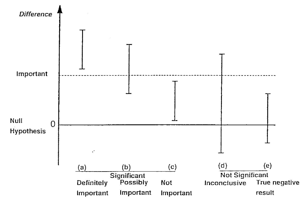
It is possible when conducting significance tests, particularly in very large studies, that a small effect is found to be statistically significant. For example, say in a large study of over 1000 patients, a new medication was found to lower blood pressure on average by 1 mmHg more than a currently accepted drug and this was statistically significant (P < 0.05). However, such a small decrease in blood pressure would probably not be considered clinically important. The cost and side effects of prescribing the new medication would need to be weighed against the very small average benefit that would be expected. In this case, although the null hypothesis would be rejected (i.e. the result is statistically significant), the result would not be clinically important. This is the situation described in scenario (c) of Figure 4.1.
Conversely, it is possible to obtain a large, clinically important difference between groups, but a P value that does not demonstrate a statistically significant difference.
For example, consider a study to measure the rate of hospital admissions. We may find that 80% of children who present to the Emergency Department are admitted before an intervention is introduced compared to only 65% of children after the intervention. However, the P value may be calculated as 0.11 and is non-significant. This is because only 60 children were surveyed in each period. Here, the reduction in the admission rate by 15% represents a clinically important difference, but not statistically significant. This situation is represented in scenario (d) of Figure 4.1.
The important thing to remember is that statistical significance does not always correspond to practical importance. A statistically significant result may be practically unimportant, and a statistically non-significant results may be practically important.
4.5 Errors in significance testing
There are two conclusions we can draw when conducting a hypothesis test: if the P-value is small, there is strong evidence against the null hypothesis and we reject the null hypothesis. If the P-value is not small, there is little evidence against the null hypothesis and we fail to reject the null hypothesis. As discussed above, the “small” cut-point for the P-value is often taken as 0.05. We refer to this value as \(\alpha\) (alpha).
We can conduct a thought experiment and compare our hypothesis test conclusion to reality. In reality, either the null hypothesis is true, or it is false. Of course, if we knew what reality was, we would not need to conduct a hypothesis test. But we can compare our possible hypothesis test conclusions to the true (unobserved) reality.
If the null hypothesis was true in reality, our hypothesis test can fail to reject the null hypothesis – this would be a correct conclusion. However, the hypothesis test could lead us to rejecting the null hypothesis – this would be an incorrect conclusion. We call this scenario a Type I error, and it has a probability of \(\alpha\).
The other situation is where, in reality, the null hypothesis is false. A correct conclusion would be where our hypothesis test rejects the null hypothesis. However, if our hypothesis test fails to reject the null hypothesis, we have made a Type II error. The probability of making a Type II error is denoted \(\beta\) (beta). We will see in Module 10 that \(\beta\) is determined by the size of the study.
The error in falsely rejecting the null hypothesis when it is true (type I error), or in falsely accepting the null hypothesis when it is not true (type II error) is summarised in Table 4.2. We will return to these concepts in Module 10, when discussing how to determine the appropriate sample size of a study.
| Effect | No effect |
|---|---|---|
Evidence | Correct | ɑ |
No evidence | β | Correct |
4.6 Confidence intervals in hypothesis testing
In Module 3, the 95% confidence interval around a mean value was calculated to show the precision of the summary statistic. The 95% confidence intervals around other summary statistics can also be calculated.
For example, if we were comparing the means of two groups, we would want to test the null hypothesis that the difference in means is zero, that there is no true difference between the groups.
From the data from the two groups, we could estimate the difference in means, the standard error of the difference in means and the 95% confidence interval around the difference. To estimate the 95% confidence interval, we use the formula given in Module 3, that is:
\[ 95\% \text{ CI} = \text{Difference in means} \pm 1.96 \times \text{SE}(\text{Difference in means)} \]
It is important to remember that the 95% CI is estimated from the standard error, and that the standard error has a direct relationship to the sample size. For small sample sizes, the standard error is large and the 95% CI becomes wider. Conversely, the larger the sample size, the smaller the standard error and the narrower the 95% CI becomes indicating a more precise estimate of the mean difference.
The 95% CI tells us the region in which we are 95% confident that the true difference between the groups in the population lies. If this region contains the null value of no difference, we can say that we are 95% confident that there is no true difference between the groups and therefore we would not reject the null hypothesis. This is shown in the top two estimates in Figure 4.2. If the zero value lies outside the 95% confidence interval, we can conclude that there is evidence of a difference between the groups because we are 95% confident that the difference does not encompass a zero value (as shown in the lower two estimates in Figure 4.2.
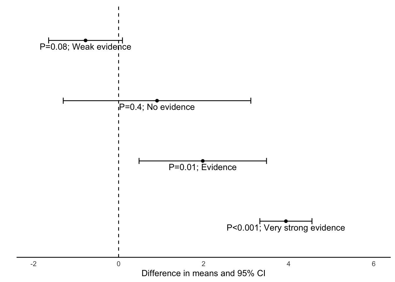
For relative risk and odds ratio measures, when the 95% CI includes the value of 1 it indicates that we can be 95% confident that the true RR or OR of the association between the study factor and outcome factor includes 1.0 in the source population. This indicates little evidence of an association between the study factor and the outcome factor, e.g. if the results of a study were reported as RR = 1.10 (95% CI 0.95 to 1.25). The P-value can be calculated to assess this (discussed in Module 7).
Type of outcome | Measure of effect | Null value |
|---|---|---|
Continuous | Difference in means | 0 |
Binary | Difference in proportions | 0 |
Binary | Relative risk | 1 |
Binary | Odds ratio | 1 |
4.7 One-sample t-test
A one-sample t-test tests whether a sample mean is different to a hypothesised value. The t-distribution and its relation to normal distribution has been discussed in detailed in Module 3.
In a one-sample t-test, a t-value is computed as the sample mean divided by the standard error of the mean. The significance of the t-value is then computed using software, or can be obtained from a statistical table.
The principles of this test can be used for applications such as testing whether the mean of a sample is different from a known population mean, for example testing whether the IQ of a group of children is different from the population mean of 100 IQ points or testing whether the number of average hours worked in an adult sample is different from the population mean of 38 hours.
Worked Example
The mean diastolic blood pressure (BP) of the general US population is known to be 71 mm Hg. The diastolic blood pressure of 733 female Pima indigenous Americans was measured and a density plot showed that the data were approximately normally distributed. The mean diastolic blood pressure in the sample was 72.4 mm Hg with a standard deviation of 12.38 mm Hg.
We can use jamovi or R to conduct a one sample t-test using the data available on Moodle (mod04_blood_pressure.csv). The results from this test are summarised below.
| n | Mean | Standard deviation | Standard error | 95% confidence interval of the mean |
|---|---|---|---|---|
| 733 | 72.4 | 12.38 | 0.46 | 71.5 to 73.3 |
The test statistic for the one-sample t-test is calculated as t732=3.07, with a P-value of 0.002.
The mean diastolic blood pressure of females from Pima is estimated as 72.4 mmHg (95% CI: 71.5 to 73.3 mmHg), which is higher than that of the general US population. Note that this interval does not contain the mean of the general US population (71 mm Hg), providing some indication that the mean diastolic blood pressure of female Pima people is higher than that of the general US population.
The result from the formal hypothesis test gives strong evidence that the mean diastolic BP of the female Pima people is higher than that of the general US population (t732=3.07, P=0.002).
4.8 One and two tailed tests
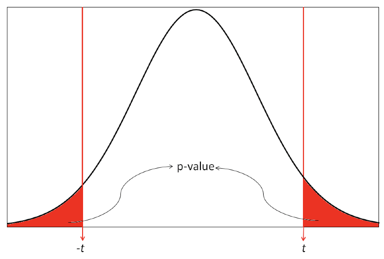
Most statistical tests are two tailed tests, that is, we conduct a test that allows for the summary statistic in the group of interest to be either higher or lower than in the comparison group. For a t-test, this requires that we obtain a two-tailed P value which gives us the probability of the t-value being in either one of the two tails of the t-distribution as shown in Figure 4.3. The shaded regions show the t values that indicate a P value less than 0.05.
Occasionally, one tailed tests are conducted in which the summary statistic in the group of interest can only be higher or lower than the comparison group, i.e. a difference is specified to occur in one direction only. In most studies, two tailed tests of significance are used to allow for the possibility that the effect size could occur in either direction. In clinical trials, this would mean allowing for a result that can indicate a benefit or an adverse effect in response to a new treatment. In epidemiological studies, two tailed tests are used to allow for the fact that exposure to a factor of interest may be adverse or may be beneficial. This conservative approach is usually adopted to prevent missing important effects that occur in the opposite direction to that expected by the researchers.
4.9 A note on P-values displayed by software
You will often see P-values generated by statistical software presented as 0.000 or 0.0000. As P-values can never be equal to zero, any P-value displayed in this way should be converted to <0.001 or <0.0001 respectively (i.e. replace the last 0 with a 1, and use the less-than symbol).
R can display P-values in a very cryptic way: \(\text{6.478546e-05}\) for example. This is translated as:
\[ \begin{aligned} 6.478546e-05 &= 6.478546 \times 10^{-5} \\ &= 6.478546 \times 0.00001 \\ &= 0.00006478546 \end{aligned} \]
Such a P-value should be presented as P<0.0001.
4.10 Decision Tree
In the following modules in this course, several formal statistical tests will be described to analyse different types of data sets that have been collected to test set null hypotheses. It is important that the correct statistical test is selected to generate P-values and estimate effect size. If an incorrect statistical test is used, the assumptions of the test may be violated, the effect size may be biased and the P value generated may be incorrect.
Selecting the correct test to use in each situation depends on the study design and the nature of the variables collected. Figure 1 in the Appendix shows a decision tree which enables you to decide the type of test to select based on the nature of the data.
Jamovi notes
4.11 One sample t-test
We will use data from mod04_blood_pressure.csv to demonstrate how a one-sample t-test is conducted in Jamovi. To perform the test, go to Analyses > T-Tests > One Sample T-Test.
Select dbp as the Dependent Variable. Enter the hypothesised mean as the Test value (71 in this example) as shown below.
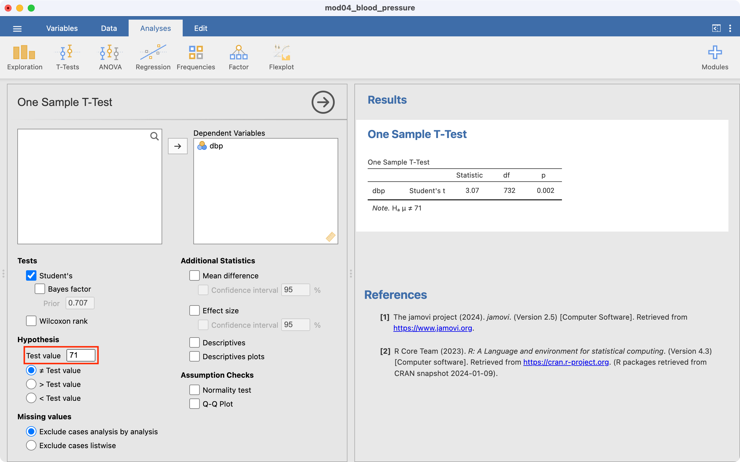
The test statistic (i.e. t and its degrees of freedom) are provided. By default, Jamovi will calculate a P-value for the two-sided test (Ha: mean \(\neq\) 71), which appropriate for this example.
Note that the one-sample t-test output does not include the mean or the 95% confidence interval of the mean of your variable of interest. This should be obtained using Exploration > Descriptives:

R notes
4.12 One sample t-test
We will use data from mod04_blood_pressure.csv to demonstrate how a one-sample t-test is conducted in R. To test whether the mean diastolic blood pressure of the population from which the sample was drawn is equal to 71, we can use the t.test command:
pima <- read.csv("data/examples/mod04_blood_pressure.csv")
t.test(pima$dbp, mu=71)
    One Sample t-test

data:  pima$dbp
t = 3.0725, df = 732, p-value = 0.002202
alternative hypothesis: true mean is not equal to 71
95 percent confidence interval:
 71.50732 73.30305
sample estimates:
mean of x
 72.40518
The output provides:
- a test statistic (t=3.07);
- degrees of freedom for the test statistic (df = 732);
- a P-value from the two-sided test (P=0.002);
- the mean of the sample (72.4);
- and the 95% confidence interval of the mean (71.5 to 73.3).
Activities
Activity 4.1
In each of the following situations, what decision should be made about the null hypothesis if the researcher indicates that:
- P < 0.01
- P > 0.05
- “ns”
- “significant differences exist”
Activity 4.2
For the following hypothetical situations, formulate the null hypothesis and alternative hypothesis and write a conclusion about the study results:
- A study was conducted to investigate whether the mean systolic blood pressure of males aged 40 to 60 years was different to the mean systolic blood pressure of females aged 40 to 60 years. The result of the study was that the mean systolic blood pressure was higher in males by 5.1 mmHg (95% CI 2.4 to 7.6; P = 0.008).
- A case-control study was conducted to investigate the association between obesity and breast cancer. The researchers found an OR of 3.21 (95% CI 1.15 to 8.47; P = 0.03).
- A cohort study investigated the relationship between eating a healthy diet and the incidence of influenza infection among adults aged 20 to 60 years. The results were RR = 0.88 (95% CI 0.65 to 1.50; P = 0.2).
Activity 4.3
A pilot study was conducted to compare the mean daily energy intake of women aged 25 to 30 years with the recommended intake of 7750 kJ/day. In this study, the average daily energy intake over 10 days was recorded for 12 healthy women of that age group. The data are in the the Excel file Activity_4.3.xlsx. Import the file into jamovi or R for this activity.
- State the research question
- Formulate the null hypothesis
- Formulate the alternative hypothesis
- Analyse the data in jamovi or R and report your conclusions
Activity 4.4
Which procedure gives the researcher the better chance of rejecting a null hypothesis?
- comparing the data-based p-value with the level of significance at 5%
- comparing the 95% CI with a nominated value
- neither procedure
Activity 4.5
Setting the significance level at P < 0.10 instead of the more usual P < 0.05 increases the likelihood of:
- a Type I error
- a Type II error
- rejecting the null hypothesis
- Not rejecting the null hypothesis
Activity 4.6
For a fixed sample size setting the significance level at a very extreme cutoff such as P < 0.001 increases the chances of: a) obtaining a significant result b) rejecting the null hypothesis c) a Type I error d) a Type II error