Learning objectives

By the end of this module you will be able to:

Describe the characteristics of a Normal distribution
Compute probabilities from a Normal distribution using statistical software
Briefly outline other types of distributions
Explain the purpose of sampling, different sampling methods and their implications for data analysis
Distinguish between standard deviation of a sample and standard error of a mean
Calculate and interpret confidence intervals for a mean

Optional readings

Kirkwood and Sterne (2001); Chapters 4, 5 and 6. [UNSW Library Link]

Bland (2015); Sections 3.3 and 3.4, Chapter 7, Sections 8.1 to 8.3. [UNSW Library Link]

3.1 Introduction

In this module, we will continue our introduction to probability by considering probability distributions for continuous data. We will introduce one of the most important distributions in statistics: the Normal distribution.

To describe the characteristics of a population we can gather data about the entire population (as is undertaken in a national census) or we can gather data from a sample of the population. When undertaking a research study, taking a sample from a population is far more cost-effective and less time consuming than collecting information from the entire population. When a sample of a population is selected, summary statistics that describe the sample are used to make inferences about the total population from which the sample was drawn. These are referred to as inferential statistics.

However, for the inferences about the population to be valid, a random sample of the population must be obtained. The goal of using random sampling methods is to obtain a sample that is representative of the target population. In other words, apart from random error, the information derived from the sample is expected to be much the same as the information collected from a complete population census as long as the sample is large enough.

3.2 Probability for continuous variables

Calculating the probability for a categorical random variable is relatively straightforward, as there are only a finite number of possible events. However, there are an infinite number of possible values for a continuous variable, and we calculate the probability that the continuous variable lies in a range of values.

3.3 Normal distribution

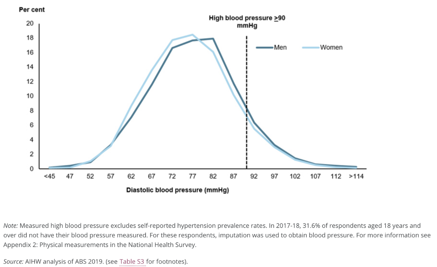
The frequency plot for many biological and clinical measurements (for example blood pressure and height) follow a bell shape where the curve is symmetrical about the mean value and has tails at either end. Figure 3.1 ¹ and Figure 3.2 ² demonstrate this type of distribution.

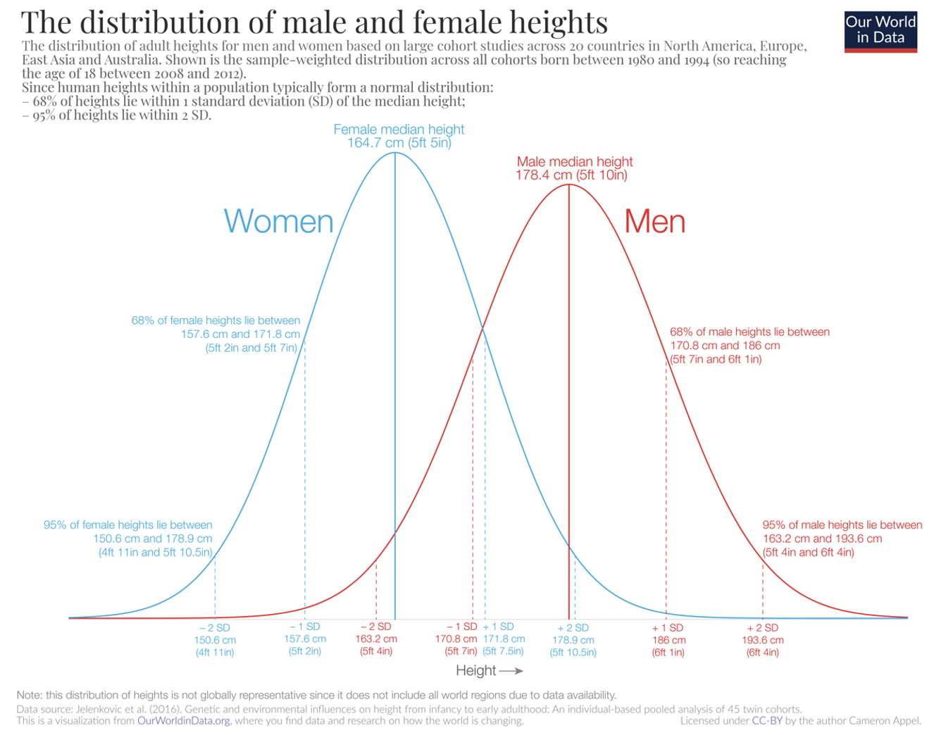
Figure 3.1: Distribution of diastolic blood pressure, 2017–18 Australian Bureau of Statistics National Health Survey

Figure 3.2: Distribution of male and female heights

The Normal distribution, also called the Gaussian distribution (named after Johann Carl Friedrich Gauss, 1777–1855), has been shown to fit the frequency distribution of many naturally occurring variables. It is characterised by its bell-shaped, symmetric curve and its tails that approach zero on either side.

There are two reasons for the importance of the Normal distribution in biostatistics (Kirkwood and Sterne, 2003). The first is that many variables can be modelled reasonably well using the Normal distribution. Even if the observed data were not Normally distributed, it can often be made reasonably Normal after applying some transformation of the data. The second (and possible most important) reason, is based on the central limit theorem and will be discussed later in this module.

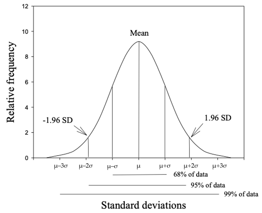
The Normal distribution is characterised by two parameters: the mean ($\mu$) and the standard deviation ($\sigma$). The mean defines where the middle of the Normal distribution is located, and the standard deviation defines how wide the tails of the distribution are.

For a Normal distribution, about 68% of the observations lie between $- \sigma$ and $\sigma$ of the mean; 95% of the observations lie between $−1.96 \times \sigma$ and $1.96 \times \sigma$ from the mean; and almost all the observations (99.7%) lie between $-3 \times \sigma$ and $3 \times \sigma$ (Figure 3.3). Also note that the mean is the same as the median, as the curve is symmetric about its mean.

Figure 3.3: Characteristics of a Normal distribution

3.4 The Standard Normal distribution

As each Normal distribution is defined by its mean and standard deviation, there are an infinite number of possible Normal distributions. However, every Normal distribution can be transformed to what we call the Standard Normal distribution, which has a mean of zero ($\mu = 0$) and a standard deviation of one ($\sigma = 1$). The Standard Normal distribution is so important that it has been assigned its own symbol: Z.

Every observation from a Normal distribution $X$ with a mean $\mu$ and a standard deviation $\sigma$ can be transformed to a z-score (also called a Standard Normal deviate) by the formula:

\[ z = \frac{x - \mu}{\sigma} \]

The z-score is simply how far an observation lies from the population mean value, scaled by the population standard deviation.

We can use z-scores to estimate probabilities, as shown in Worked Example 2.2.

Worked Example

This example extends the example of diastolic blood pressure shown in Figure 3.1. Assume that the mean diastolic blood pressure for men is 77.9 mmHg, with a standard deviation of 11. What is the probability that a man selected at random will have high blood pressure (i.e. diastolic blood pressure ≥ 90)?

To estimate the probability that diastolic blood pressure ≥ 90 (i.e. the upper tail probability), we first need to calculate the z-score that corresponds to 90 mmHg.

Using the z-score formula, with x=90, $\mu$=77.9 and $\sigma$=11:

\[ z = \frac{90 - 77.9}{11} = 1.1 \] Thus, a blood pressure of 90 mmHg corresponds to a z-score of 1.1, or a value 1.1 $\times \sigma$ above the mean weight of the population.

Figure 3.4 shows the probability of a diastolic blood pressure of 90 mmHg or more in the population for a z-score of greater than 1.1 on a Standard Normal distribution.

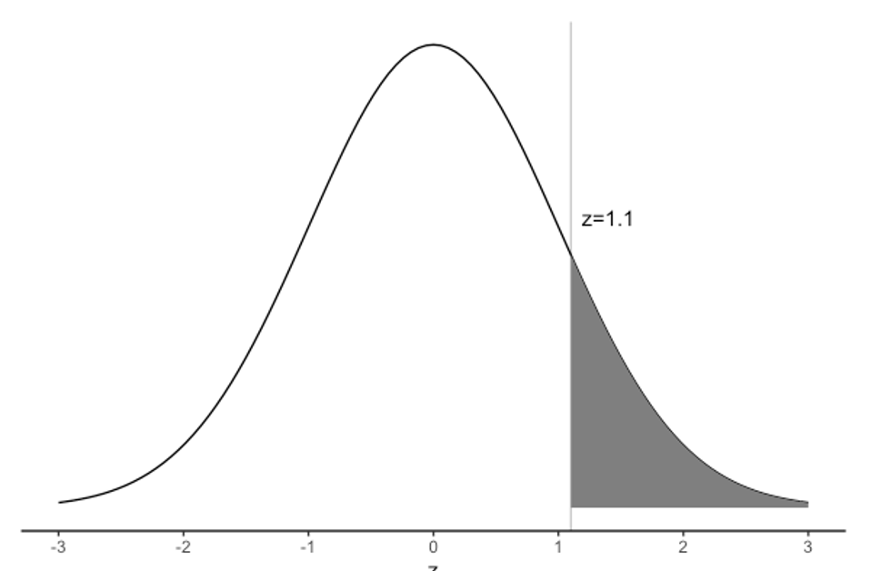
Figure 3.4: Area under the Standard Normal curve (as probability) for Z > 1.1

Using software, we find the probability that a person has a diastolic blood pressure of 90 mmHg or more as P(Z ≥ 1.1) = 0.136.

Apart from calculating probabilities, z-scores are most useful for comparing measurements taken from a sample to a known population distribution. It allows measurements to be compared to one another despite being on different scales or having different predicted values.

For example, if we take a sample of children and measure their weights, it is useful to describe those weights as z-scores from the population weight distribution for each age and gender. Such distributions from large population samples are widely available. This allows us to describe a child’s weight in terms of how much it is above or below the population average. For example, if mean weights were compared, children aged 5 years would be on average heavier than the children aged 3 years simply because they are older and therefore larger. To make a valid comparison, we could use the Z-scores to say that children aged 3 years tend to be more overweight than children aged 5 years because they have a higher mean z-score for weight.

3.5 Assessing Normality

There are several ways to assess whether a continuous variable is Normally distributed. The best way to assess whether a variable is Normally distributed is to plot its distribution, using a density plot for example. If the density plot looks appoximately bell-shaped and approximately symmetrical, assuming Normality would be reasonable.

It may be useful to examine a boxplot of a variable in conjunction with a density plot. However a boxplot in isolation is not as useful as a density plot, as a boxplot only indicates whether a variable is distributed symmetrically (indicated by equal “whiskers”). A boxplot cannot give an indication of whether the distribution is bell-shaped, or flat.

For your information: There are formal tests that test for Normality. These tests are beyond the scope of this course and are not recommended.

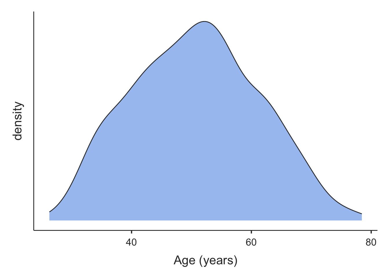
We can construct a density plot for age in the pbc data introduced in Module 1. We can see that the density plot is approximately approximately bell-shaped and roughly symmetrical. The mean (50.7 years) and median (51 years) are similar, as would be expected for a Normal distribution. Thus, it would be reasonable to assume that age is Normally distributed in this set of data.

Figure 3.5: Density plot of participant age from PBC study data

3.6 Non-Normally distributed measurements

Not all measurements are Normally distributed, and the symmetry of the bell shape may be distorted by the presence of some very small or very large values. Non-Normal distributions such as this are called skewed distributions.

When there are some very large values, the distribution is said to be positively skewed.This often occurs when measuring variables related to time, such as days of hospital stay, where most patients have short stays (say 1 - 5 days) but a few patients with serious medical conditions have very long lengths of hospital stay (say 20 - 100 days).

In practice, most parametric summary statistics are quite robust to minor deviations from Normality and non-parametric statistical methods are only required when the sample size is small and/or the data are obviously skewed with some influential outliers.

When the data are markedly skewed, density plots are not all bell-shaped. For example, serum bilirubin measured from participants in the PBC study are presented in Figure 3.6.

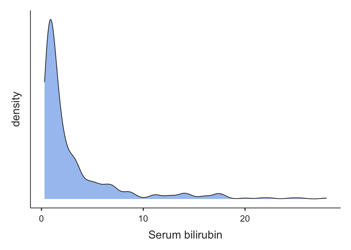
Figure 3.6: Density plot of serum bilirubin from PBC study data

In the plot of Figure 3.6, there is a tail of values to the right, so we would conclude that the distribution is skewed to the right. The mean (3.2 mg/dL) is much larger than the median (1.4 mg/dL), as expected from a skewed distribution.

3.7 Parametric and non-parametric statistical methods

Many statistical methods are based on assumptions about the distribution of the variable – these methods are known as parametric statistical methods. Many methods of statistical inferences based on theoretical sampling properties that are derived from a Normal distribution with the characteristics described above. Thus, it is important that measurements approximate to a Normal distribution before these parametric methods are used. The methods are called ‘parametric’ because they are based on the parameters – the mean and standard deviation - that underlie a Normal distribution. Statistics which do not assume a particular distribution are called distribution-free statistics, or ‘non-parametric statistics’.

In this course, you will learn about both parametric and non-parametric statistical methods. Parametric summary statistical methods include those based on the mean, standard deviation and range (Module 1), and standard error and 95% confidence interval (Module 3). Parametric statistical tests also include t-tests which will be covered in Modules 4 and 5, and correlation and regression described in Module 8.

Non-parametric summary statistical methods are often based on ranks, and may use such statistics as the median, mode and inter-quartile range (Module 1). Non-parametric statistical tests that use ranking are described in Module 9.

3.8 Other types of probability distributions

In this module we have considered a Normal probability distribution and how to use it to measure the precision of continuously distributed measurements. Data also follow other types of distributions which are briefly described below. In other modules in this course, we will be looking at a range of methods to analyse health data and will refer back to these different distributions.

Normal approximation of binomial: When the sample size becomes large, it becomes cumbersome to calculate the exact probability of an event using the binomial distribution. Conveniently, with large sample sizes, the binomial distribution approximates a Normal distribution. The mean and SD of a binomial distribution can be used to calculate the probability of the event as though it was from a Normal distribution.

Poisson distribution: is another distribution which is often used in health research for modelling count data. The Poisson distribution is followed when a number of events happen in a fixed time interval. This distribution is useful for describing data such as deaths in the population in a time period. For example, the number of deaths from breast cancer in one year in women over 50 years old will be an observation from a Poisson distribution. We can also use this to make comparisons of mortality rates between populations.

Many other probability distributions can be derived for functions which arise in statistical analyses but the chi-squared, t and F distributions are the three distributions that are most widely used. These have many applications, some of which are described in later modules.

The chi-squared distribution is a skewed distribution which allows us to determine the probability of a deviation between a count that we observe and a count that we expect for categorical data. One use of this is in conducting statistical tests for categorical data. See Module 7.

A t-distribution is used when the population standard deviation is not known. The t-distribution is appropriate for small samples (<30) and its distribution is bell shaped similar to a Normal distribution but slightly flatter. The t-distribution is useful for comparing mean values. See Module 4 and Module 5.

3.9 Sampling methods

Methods have been designed to select participants from a population such that each person in the target population has an equal probability of being chosen. Methods that use this approach are called random sampling methods. Examples include simple random sampling and stratified random sampling.

In simple random sampling, every person in the population from which the sample is drawn has the same random chance of being selected into the sample. To implement this method, every person in the population is allocated an ID number and then a random sample of the ID numbers is selected. Software packages can be used to generate a list of random numbers to select the random sample.

In stratified sampling, the population is divided into distinct non-overlapping subgroups (strata) according to an important characteristic (e.g. age or sex) and then a random sample is selected from each of the strata. This method is used to ensure that sufficient numbers of people are sampled from each stratum and therefore each subgroup of interest is adequately represented in the sample.

The purpose of using random sampling is to minimise selection bias to ensure that the sample enrolled in a study is representative of the population being studied. This is important because the summary statistics that are obtained can then be regarded as valid in that they can be applied (generalised) back to the population.

A non-representative sample might occur when random sampling is used, simply by chance. However, non-random sampling methods, such as using a study population that does not represent the whole population, will often result in a non-representative sample being selected so that the summary statistics from the sample cannot be generalised back to the population from which the participants were drawn. The effects of non-random error are much more serious than the effects of random error. Concepts such as non-random error (i.e. systematic bias), selection bias, validity and generalisability are discussed in more detail in PHCM9794: Foundations of Epidemiology.

3.10 Standard error and precision

Module 1 introduced the mean, variance and standard deviation as measures of central tendency and spread for continuous measurements from a sample or a population. As described in Module 1, we rarely have data on the entire population but we infer information about the population from a sample. For example, we use the sample mean $\bar x$ as an estimate of the true population mean $\mu$.

However, a sample taken from a population is usually a small proportion of the total population. If we were to take multiple samples of data and calculate the sample mean for each sample, we would not expect them to be identical. If our samples were very small, we would not be surprised if our estimated sample means were somewhat different from each other. However, if our samples were large, we would expect the sample means to be less variable, i.e. the estimated sample means would be more close to each other, and hopefully, to the true population mean.

The standard error of the mean

A point estimate is a single best guess of the true value in the population - taken from our sample of data. Different samples will provide slightly different point estimates. The standard error is a measure of variability of the point estimate.

In particular, the standard error of the mean measures the extent to which we expect the means from different samples to vary because of chance due to the sampling process. This statistic is directly proportional to the standard deviation of the variable, and inversely proportional to the size of the sample. The standard error of the mean for a continuously distributed measurement for which the SD is an accurate measure of spread is computed as follows:

\[ \text{SE}(\bar{x}) = \frac{\text{SD}}{\sqrt{n}} \]

Take for example, a set of weights of students attending a university gym in a particular hour. The thirty weights are given below:

Table 3.1: Weight of 30 gym attendees

65.0	70.0	70.0	67.5	65.0	80.0
70.0	72.5	67.5	62.5	67.5	72.5
60.0	65.0	72.5	77.5	75.0	75.0
75.0	70.0	67.5	77.5	67.5	62.5
75.0	62.5	70.0	75.0	72.5	70.0

We can calculate the mean (70.0kg) and the standard deviation (5.04kg). Hence, the standard error of the mean is estimated as:

\[ \text{SE}(\bar{x}) = \frac{5.04}{\sqrt{30}} = 0.92 \] Because the calculation uses the sample size (n) (i.e. the number of study participants) in the denominator, the SE will become smaller when the sample size becomes larger. A smaller SE indicates that the estimated mean value is more precise.

The standard error is an important statistic that is related to sampling variation. When a random sample of a population is selected, it is likely to differ in some characteristic compared with another random sample selected from the same population. Also, when a sample of a population is taken, the true population mean is an unknown value.

Just as the standard deviation measures the spread of the data around the population mean, the standard error of the mean measures the spread of the sample means. Note that we do not have different samples, only one. It is a theoretical concept which enables us to conduct various other statistical analyses.

3.11 Central limit theorem

Even though we now have an estimate of the mean and its standard error, we might like to know what the mean from a different random sample of the same size might be. To do this, we need to know how sample means are distributed. In determining the form of the probability distribution of the sample mean ($\bar{x}$), we consider two cases:

When the population distribution is unknown:

The central limit theorem for this situation states:

In selecting random samples of size $n$ from a population with mean $\mu$ and standard deviation $\sigma$, the sampling distribution of the sample mean $\bar{x}$ approaches a normal distribution with mean $\mu$ and standard deviation $\tfrac{\sigma}{\sqrt{n}}$ as the sample size becomes large.

The sample size n = 30 and above is a rule of thumb for the central limit theorem to be used. However, larger sample sizes may be needed if the distribution is highly skewed.

When the population is assumed to be normal:

In this case the sampling distribution of $\bar{x}$ is normal for any sample size.

3.12 95% confidence interval of the mean

Earlier, we showed that the characteristics of a Standard Normal Distribution are that 95% of the data lie within 1.96 standard deviations from the mean (Figure 3.2). Because the central limit theorem states that the sampling distribution of the mean is approximately Normal in large enough samples, we expect that 95% of the mean values would fall within 1.96 × SE units above and below the measured mean population value.

For example, if we repeated the study on weight 100 times using 100 different random samples from the population and calculated the mean weight for each of the 100 samples, approximately 95% of the values for the mean weight calculated for each of the 100 samples would fall within 1.96 × SE of the population mean weight.

This interpretation of the SE is translated into the concept of precision as a 95% confidence interval (CI). A 95% CI is a range of values within which we have 95% confidence that the true population mean lies. If an experiment was conducted a very large number of times, and a 95%CI was calculated for each experiment, 95% of the confidence intervals would contain the true population mean.

The calculation of the 95% CI for a mean is as follows:

\[ \bar{x} \pm 1.96 \times \text{SE}( \bar{x} ) \] This is the generic formula for calculating 95% CI for any summary statistic. In general, the mean value can be replaced by the point estimate of a rate or a proportion and the same formula applies for computing 95% CIs, i.e.

\[ 95\% \text{ CI} = \text{point estimate} \pm 1.96 \times \text{SE}(\text{point estimate)} \]

The main difference in the methods used to calculate the 95% CI for different point estimates is the way the SE is calculated. The methods for calculating 95% CI around proportions and other ratio measures will be discussed in Module 6.

The use of 1.96 as a general critical value to compute the 95% CI is determined by sampling theory. For the confidence interval of the mean, the critical value (1.96) is based on normal distribution (true when the population SD is known). However, in practice, statistical packages will provide slightly different confidence intervals because they use a critical value obtained from the t-distribution. The t-distribution approaches a normal distribution when the sample size approaches infinity, and is close to a normal distribution when the sample size is ≥30.The critical values obtained from the t-distribution are always larger than the corresponding critical value from the normal distribution. The difference gets smaller as the sample size becomes larger. For example, when the sample size n=10, the critical value from the t-distribution is 2.26 (rather than 1.96); when n= 30, the value is 2.05; when n=100, the value is 1.98; and when n=1000, the critical value is 1.96.

The critical value multiplied by SE (for normal distribution, 1.96 × SE) is called the maximum likely error for 95% confidence.

The t-distribution and when should I use it?

The population standard deviation ($\sigma$) is required for calculation of the standard error. Usually, $\sigma$ is not known and the sample standard deviation ($s$) is used to estimate it. It is known, however, that the sample standard deviation of a normally distributed variable underestimates the true value of $\sigma$, particularly when the sample size is small.

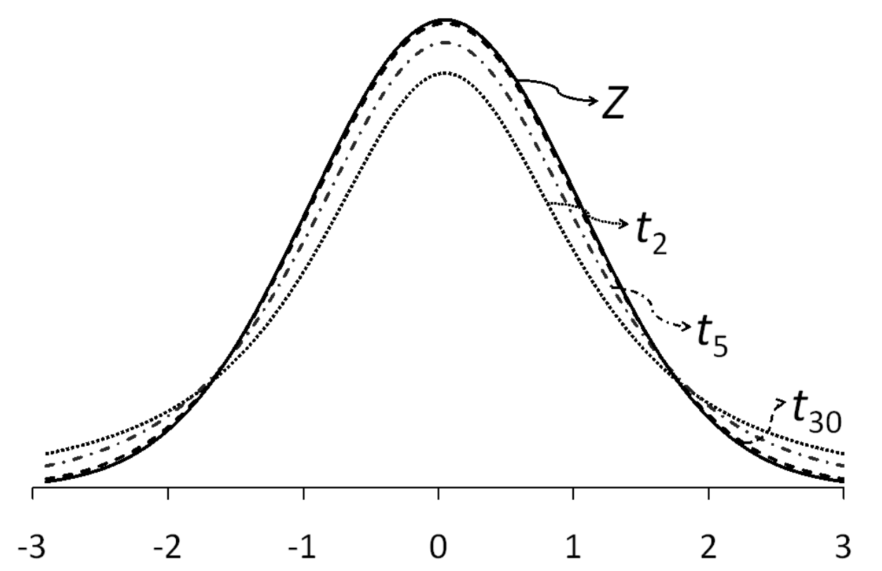
Someone by the pseudonym of Student came up with the Student’s t distribution with ($n-1$) degrees of freedom to account for this underestimation. It looks very much like the standardised normal distribution, only that it has fatter tails (Figure 3.7). As the degrees of freedom increase (i.e. as $n$ increases), the t-distribution gradually approaches the standard normal distribution. With a sufficiently large sample size, the Student’s t-distribution closely approximates the standardised normal distribution.

Figure 3.7: The normal (Z) and the student’s t-distribution with 2, 5 and 30 degrees of freedom

If a variable $X$ is normally distributed and the population standard deviation $\sigma$ is known, using the normal distribution is appropriate. However, if $\sigma$ is not known then one should use the student t-distribution with ($n – 1$) degrees of freedom.

Worked Example 3.1: 95% CI of a mean using individual data

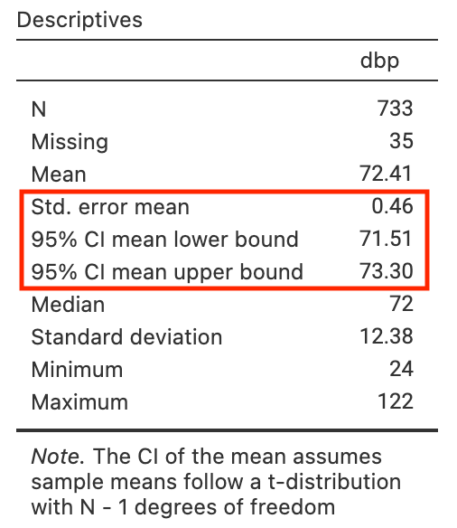
The diastolic blood pressure of 733 female Pima indigenous Americans was measured, and a density plot showed that the data were approximately normally distributed. The mean diastolic blood pressure in the sample was 72.4 mmHg with a standard deviation of 12.38 mmHg. These data are saved as mod03_blood_pressure.csv.

Use Jamovi or R, we can calculate the mean, its Standard Error, and the 95% confidence interval:

Table 3.2: Summary of blood pressure from female Pima indigenous Americans

n	Mean	Standard deviation	Standard error of the mean	95% confidence interval of the mean
733	72.4	12.38	0.46	71.5 to 73.3

We can interpret this confidence interval as: we are 95% confident that the true mean of female Pima indigenous Americans lies between 71.5 and 73.3 mmHg.

Worked Example 3.2: 95% CI of a mean using summarised data

The publication of a study using a sample of 242 participants reported a sample mean systolic blood pressure of 128.4 mmHg and a sample standard deviation of 19.56 mmHg. Find the 95% confidence interval for the mean systolic blood pressure.

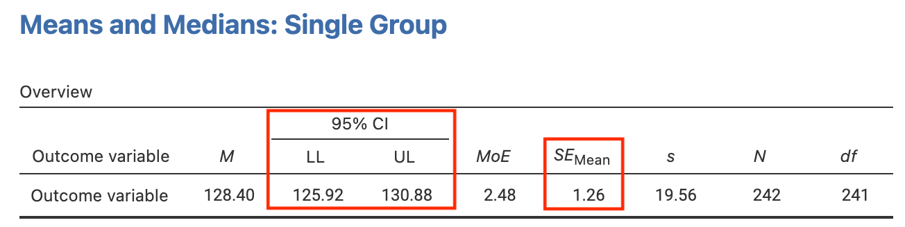
Using jamovi or R, we obtain a 95% confidence interval from 125.9232 to 130.8768.

We are 95% confident that the true mean systolic blood pressure of the population from which the sample was drawn lies between 125.9 kg and 130.9 mmHg.

Jamovi notes

3.13 Generating new variables

We commonly need to create new variables based on existing variables in our data. For example, body size is often summarised using the Body Mass Index (BMI). BMI is calculated as: $\frac{\text{weight (kg)}}{\text{height (m)}^2}$.

In this demonstration, we will import a selection of records from a large health survey, stored in the file mod03_health_survey.xlsx. The health survey data contains 1140 records, comprising:

sex: 1 = respondent identifies as male; 2 = respondent identifies as female
height: height in meters
weight: weight in kilograms

To generate a new variable, we use Data > Compute:

click Data to open the spreadsheet, and click into an empty column
click Setup then NEW COMPUTED VARIABLE
enter the name of the new variable, here BMI
in the formula (*f_x) box enter: weight / height^2 (note: ^2 represents “to the power of 2”, or “squared”)

You should check the construction of any new variable buy examining a density plot and/or a boxplot:

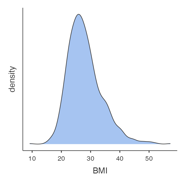
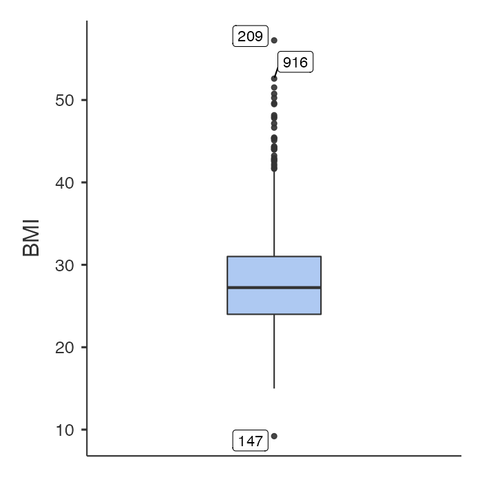
In the general population, BMI ranges between about 15 to 30. It appears that BMI has been correctly generated in this example, perhaps with some unsual values that might require investigation.

3.14 Summarising data by another variable

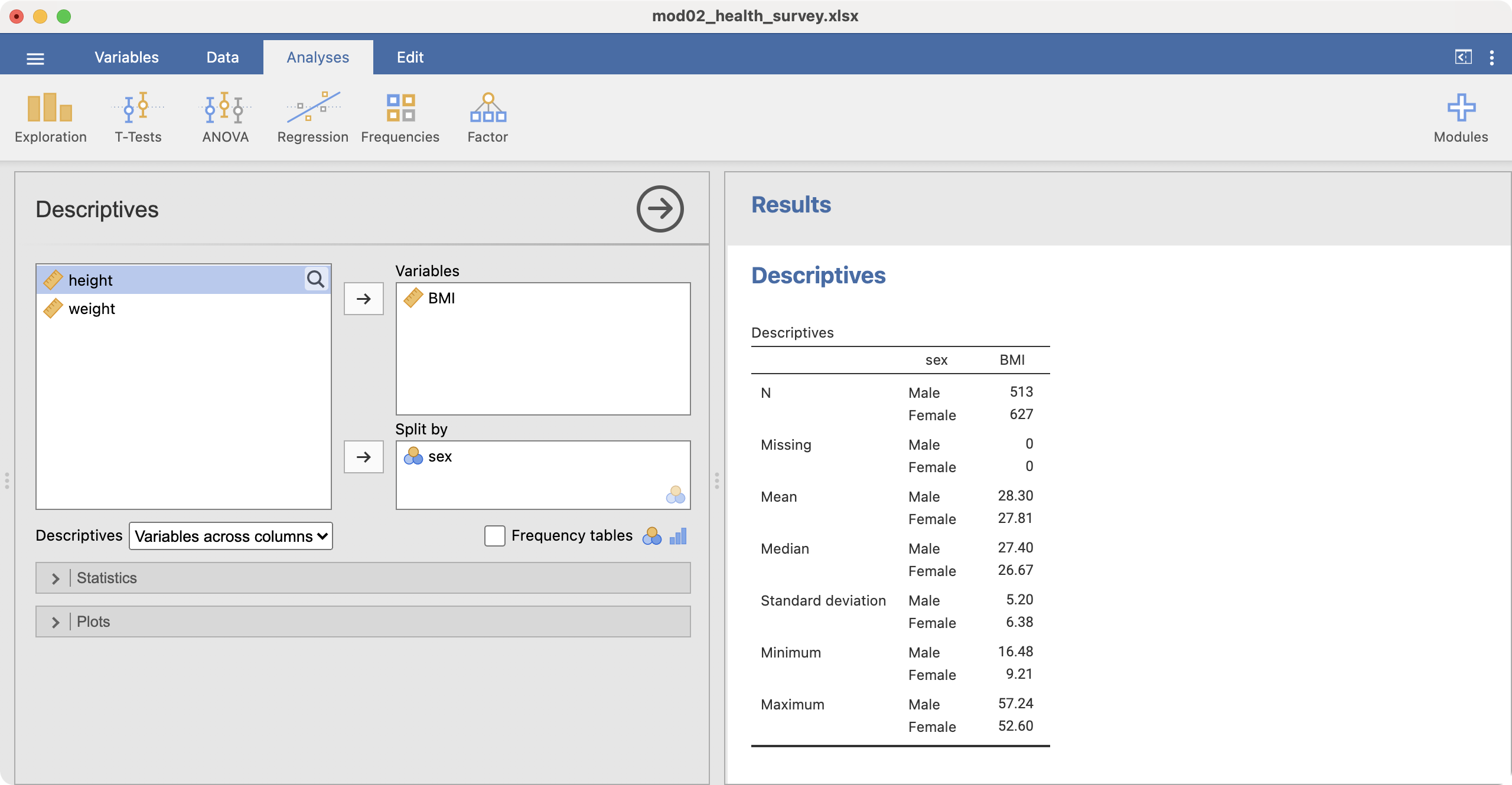
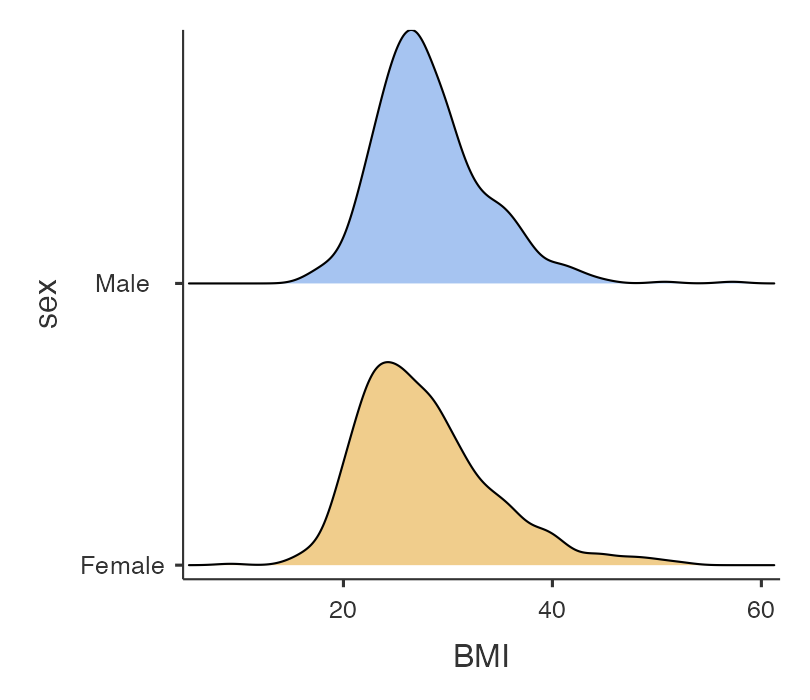
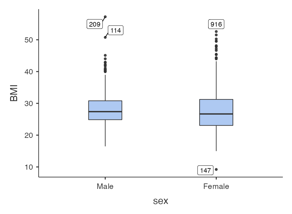
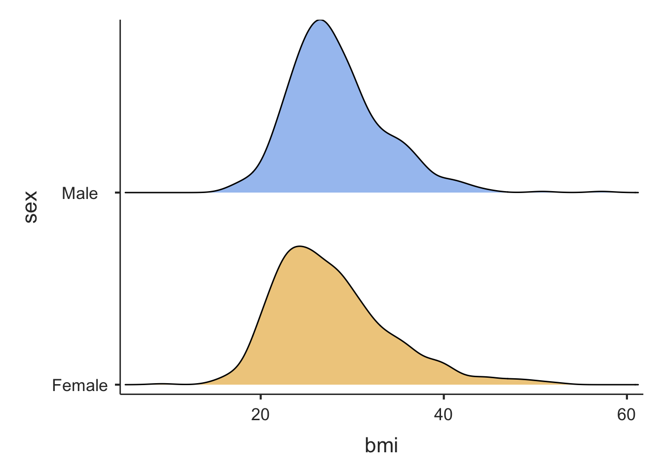
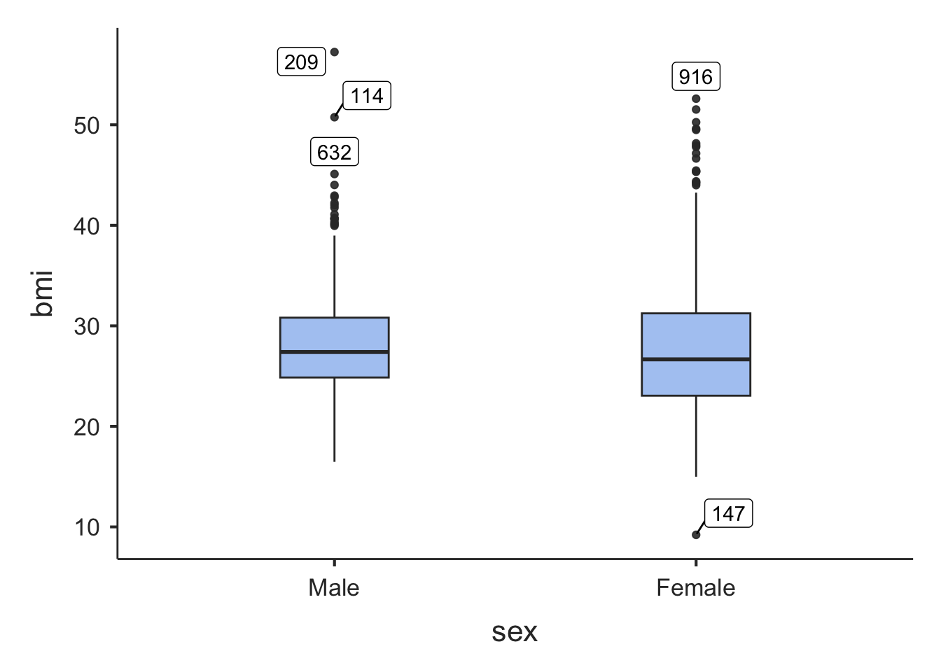
We will often want to calculate the same summary statistics by another variable. For example, we might want to calculate summary statistics for BMI for males and females separately. We can do this in jamovi by defining sex as a by-variable.

This can be done easily in jamovi by defining a Split by variable. For example, to summarise BMI for males and females separately, we use sex as the Split by variable:

3.15 Computing probabilities from a Normal distribution

jamovi does not have a point-and-click method for computing probabilities from a Normal distribution. Here, instructions are provided for using a third-party applet. This Normal Distribution Applet has been posted at https://homepage.stat.uiowa.edu/~mbognar/applets/normal.html, and provides a simple and intuitive way to compute probabilities from a Normal distribution. The applet requires three pieces of information:

$\mu$: the mean of the Normal distribution being considered
$\sigma$: the standard deviation of the Normal distribution being considered
$x$: the value being considered

We also need to consider whether we are interested in the probability being greater than x, or less than x.

For example, to obtain the probability of obtaining 0.5 or greater from a standard normal (i.e. $/mu$=0, $/sigma$=1) distribution:

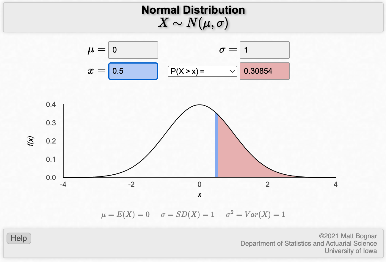
The Normal curve of interest is shaded, and the probability is provided as 0.30854.

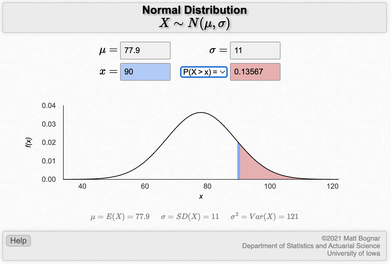
To calculate the worked example: Assume that the mean diastolic blood pressure for men is 77.9 mmHg, with a standard deviation of 11. What is the probability that a man selected at random will have high blood pressure (i.e. diastolic blood pressure greater than or equal to 90)?

3.16 Calculating a 95% confidence interval of a mean: Individual data

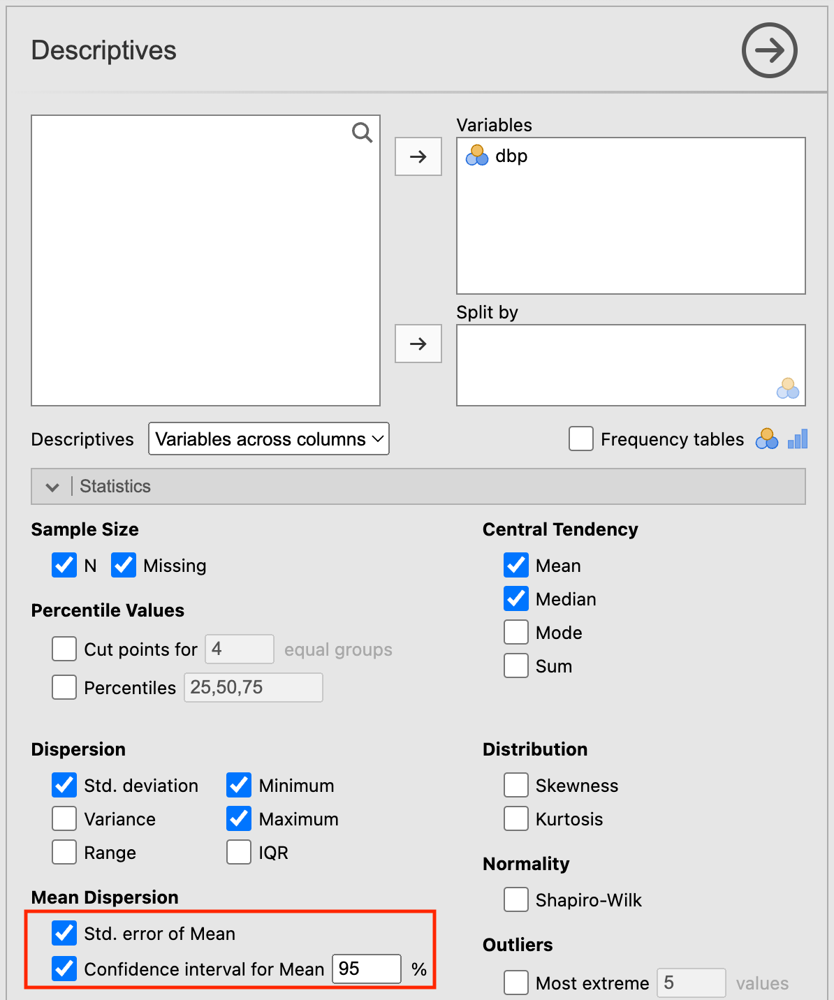
To demonstrate the computation of the 95% confidence interval of a mean, we can use the data from mod03_blood_pressure.csv. We can use Exploration > Descriptives to calculate the mean, its standard error and the 95% confidence interval for the mean. Choose dbp as the analysis variable, and select Std. error of Mean and Confidence interval for Mean in the Statistics section:

The descriptives output appears:

3.17 Calculating a 95% confidence interval of a mean: Summarised data

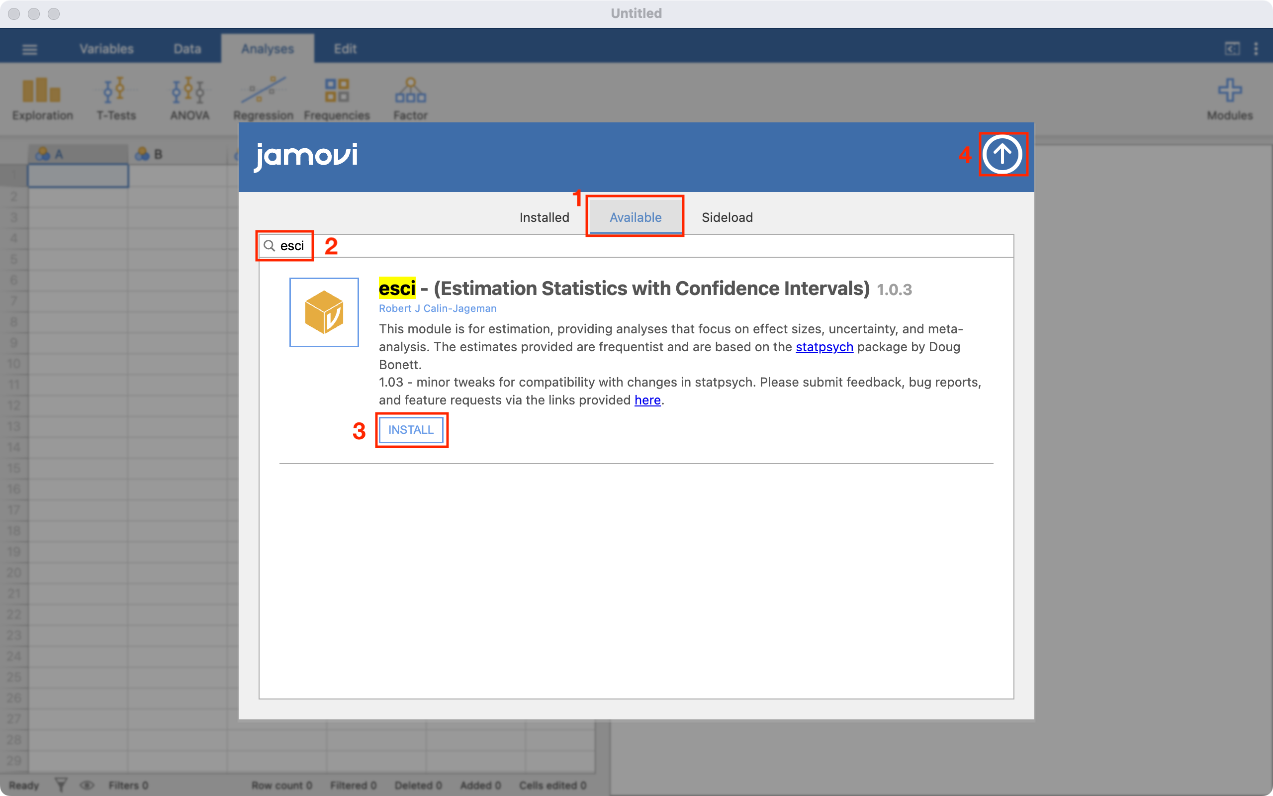
For Worked Example 3.2 where we are given the sample mean, sample standard deviation and sample size, we need to install a new Jamovi module, called esci. To install a new module, click the large + Modules button on the right-hand side of the Jamovi window, and then choose jamovi library:

To install a new module:

1 - Ensure that the middle tab, Available is selected; 2 - Type esci in the search bar. The esci module will appear; 3 - Click INSTALL to install the module 4 - Click the up-arrow to exit from the Install Module window

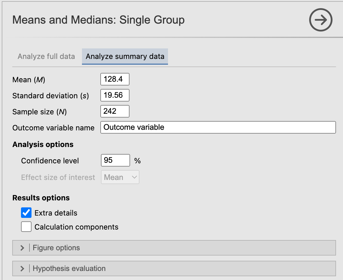
To calculate the 95% confidence interval, choose esci > Means and Medians > Single Group. Select the Analyze summary data tab, and enter the known information: here 128.4 as the Mean, 19.56 as the Standard deviation and 242 as the Sample size. Choose Extra details to obtain the Standard Error of the mean:

The 95% confidence interval is listed as the lower limit (LL) and the upper limit (UL):

R notes

3.18 Importing Excel data into R

Another common type of file that data are stored in is a Microsoft Excel file (.xls or .xlsx). In this demonstration, we will import a selection of records from a large health survey, stored in the file mod03_health_survey.xlsx.

The health survey data contains 1140 records, comprising:

sex: 1 = respondent identifies as male; 2 = respondent identifies as female
height: height in meters
weight: weight in kilograms

To import data from Microsoft Excel, we can use the read_excel() function in the readxl package.

library(readxl)

survey <- read_excel("data/examples/mod03_health_survey.xlsx")
summary(survey)

      sex           height          weight      
 Min.   :1.00   Min.   :1.220   Min.   : 22.70  
 1st Qu.:1.00   1st Qu.:1.630   1st Qu.: 68.00  
 Median :2.00   Median :1.700   Median : 79.40  
 Mean   :1.55   Mean   :1.698   Mean   : 81.19  
 3rd Qu.:2.00   3rd Qu.:1.780   3rd Qu.: 90.70  
 Max.   :2.00   Max.   :2.010   Max.   :213.20

We can see that sex has been entered as a numeric variable. We should transform it into a factor so that we can assign labels to each category:

survey$sex <- factor(survey$sex, level=c(1,2), labels=c("Male", "Female"))

summary(survey$sex)

  Male Female 
   513    627

We also note that height looks like it has been entered as meters, and weight as kilograms.

3.19 Generating new variables

Our health survey data contains information on height and weight. We often summarise body size using BMI: body mass index which is calculated as: $\frac{\text{weight (kg)}}{(\text{height (m)})^2}$

We can create a new column in our data frame in many ways, such as using the following approach:

dataframe$new_column <- <formula>

For example:

survey$bmi <- survey$weight / (survey$height^2)

We should check the construction of the new variable by examining some records. The head() and tail() functions list the first and last 6 records in any dataset.

head(survey)

# A tibble: 6 × 4
  sex    height weight   bmi
  <fct>   <dbl>  <dbl> <dbl>
1 Male     1.63   81.7  30.8
2 Male     1.63   68    25.6
3 Male     1.85   97.1  28.4
4 Male     1.78   89.8  28.3
5 Male     1.73   70.3  23.5
6 Female   1.57   85.7  34.8

tail(survey)

# A tibble: 6 × 4
  sex    height weight   bmi
  <fct>   <dbl>  <dbl> <dbl>
1 Female   1.65   95.7  35.2
2 Male     1.8    79.4  24.5
3 Female   1.73   83    27.7
4 Female   1.57   61.2  24.8
5 Male     1.7    73    25.3
6 Female   1.55   91.2  38.0

We should also check the construction of any new variable buy examining a density plot and/or a boxplot:

descriptives(data=survey, vars=bmi, dens=TRUE, box=TRUE)

In the general population, BMI ranges between about 15 to 30. It appears that BMI has been correctly generated in this example. We should investigate the very low and some of the very high values of BMI, but this will be left for another time.

3.20 Summarising data by another variable

library(jmv)
descriptives(data=survey, vars=bmi, splitBy = sex, dens=TRUE, box=TRUE)


 DESCRIPTIVES

 Descriptives                                 
 ──────────────────────────────────────────── 
                         sex       bmi        
 ──────────────────────────────────────────── 
   N                     Male           513   
                         Female         627   
   Missing               Male             0   
                         Female           0   
   Mean                  Male      28.29561   
                         Female    27.81434   
   Median                Male      27.39592   
                         Female    26.66667   
   Standard deviation    Male      5.204975   
                         Female    6.380523   
   Minimum               Male      16.47519   
                         Female    9.209299   
   Maximum               Male      57.23644   
                         Female    52.59516   
 ────────────────────────────────────────────

3.21 Summarising a single column of data

In Module 1, we started with a very simple analysis: reading in six ages, and them using summary() to calculate descriptive statistics. We then went on to use the decriptives() function in the jmv package as more flexible way of calculating descriptive statistics. Let’s revisit this analysis:

# Author: Timothy Dobbins
# Date: 5 April 2022
# Purpose: My first R script
library(jmv)

age <- c(20, 25, 23, 29, 21, 27)

# Use "summary" to obtain descriptive statistics
summary(age)

   Min. 1st Qu.  Median    Mean 3rd Qu.    Max. 
  20.00   21.50   24.00   24.17   26.50   29.00

# Use the "descriptives" function from jmv to obtain descriptive statistics
descriptives(age)

Error: Argument 'data' must be a data frame

The summary() function has worked correctly, but the descriptives() function has given an error: Error: Argument 'data' must be a data frame. What on earth is going on here?

The error gives us a clue here - the descriptives() function requires a data frame for analysis. We have provided the object age: a vector. As we saw in Section 1.12.6.3, a vector is a single column of data, while a data frame is a collection of columns.

In order to summarise a vector using the descriptives() function, we must first convert the vector into a data frame using as.data.frame(). For example:

# Author: Timothy Dobbins
# Date: 5 April 2024
# Purpose: My first R script
library(jmv)

age <- c(20, 25, 23, 29, 21, 27)

# Use "summary" to obtain descriptive statistics
summary(age)

   Min. 1st Qu.  Median    Mean 3rd Qu.    Max. 
  20.00   21.50   24.00   24.17   26.50   29.00

# Create a new data frame from the vector age:

age_df <- as.data.frame(age)

# Use "descriptives" to obtain descriptive statistics for age_df
descriptives(age_df)


 DESCRIPTIVES

 Descriptives                       
 ────────────────────────────────── 
                         age        
 ────────────────────────────────── 
   N                            6   
   Missing                      0   
   Mean                  24.16667   
   Median                24.00000   
   Standard deviation    3.488075   
   Minimum               20.00000   
   Maximum               29.00000   
 ──────────────────────────────────

3.22 Computing probabilities from a Normal distribution

We can use the pnorm function to calculate probabilities from a Normal distribution:

pnorm(q, mean, sd) calculates the probability of observing a value of q or less, from a Normal distribution with a mean of mean and a standard deviation of sd. Note that if mean and sd are not entered, they are assumed to be 0 and 1 respectively (i.e. a standard normal distribution.)
pnorm(q, mean, sd, lower.tail=FALSE) calculates the probability of observing a value of more than q, from a Normal distribution with a mean of mean and a standard deviation of sd.

To obtain the probability of obtaining 0.5 or greater from a standard normal distribution:

pnorm(0.5, lower.tail = FALSE)

[1] 0.3085375

pnorm(90, mean = 77.9, sd = 11, lower.tail = FALSE)

[1] 0.1356661

3.23 Calculating a 95% confidence interval of a mean: individual data

To demonstrate the computation of the 95% confidence interval of a mean, we can use the data from mod03_blood_pressure.csv:

pima <- read.csv("data/examples/mod03_blood_pressure.csv")

We can examine the data set using the summary command:

summary(pima)

      dbp        
 Min.   : 24.00  
 1st Qu.: 64.00  
 Median : 72.00  
 Mean   : 72.41  
 3rd Qu.: 80.00  
 Max.   :122.00

The mean and its 95% confidence interval can be obtained many ways in R. We will use the descriptives() function within the jmv package to calculate the standard error of the mean, and a confidence interval, by including se = TRUE and ci = TRUE:

library(jmv)
descriptives(data=pima, vars=dbp, se=TRUE, ci=TRUE)


 DESCRIPTIVES

 Descriptives                             
 ──────────────────────────────────────── 
                              dbp         
 ──────────────────────────────────────── 
   N                                733   
   Missing                            0   
   Mean                        72.40518   
   Std. error mean            0.4573454   
   95% CI mean lower bound     71.50732   
   95% CI mean upper bound     73.30305   
   Median                            72   
   Standard deviation          12.38216   
   Minimum                           24   
   Maximum                          122   
 ──────────────────────────────────────── 
   Note. The CI of the mean assumes
   sample means follow a
   t-distribution with N - 1 degrees
   of freedom

3.24 Calculating a 95% confidence interval of a mean: summarised data

For Worked Example 3.2 where we are given the sample mean, sample standard deviation and sample size. R does not have a built-in function to calculate a confidence interval from summarised data, but we can write our own.

Note: writing your own functions is beyond the scope of this course. You should copy and paste the code provided to do this.

### Copy this section
ci_mean <- function(n, mean, sd, width=0.95, digits=3){
  lcl <- mean - qt(p=(1 - (1-width)/2), df=n-1) * sd/sqrt(n)
  ucl <- mean + qt(p=(1 - (1-width)/2), df=n-1) * sd/sqrt(n)
  
  print(paste0(width*100, "%", " CI: ", format(round(lcl, digits=digits), nsmall = digits),
               " to ", format(round(ucl, digits=digits), nsmall = digits) ))

}
### End of copy

ci_mean(n=242, mean=128.4, sd=19.56, width=0.95)

[1] "95% CI: 125.923 to 130.877"

ci_mean(n=242, mean=128.4, sd=19.56, width=0.99)

[1] "99% CI: 125.135 to 131.665"

Activities

Activity 3.1

An investigator wishes to study people living with agoraphobia (fear of open spaces). The investigator places an advertisement in a newspaper asking for volunteer participants. A total of 100 replies are received of which the investigator randomly selects 30. However, only 15 volunteers turn up for their interview.

Which of the following statements is true?

The final 15 participants are likely to be a representative sample of the population available to the investigator
The final 15 participants are likely to be a representative sample of the population of people with agoraphobia
The randomly selected 30 participants are likely to be a representative sample of people with agoraphobia who replied to the newspaper advertisement
None of the above

The basic problem confronted by the investigator is that:

The accessible population might be different from the target population
The sample has been chosen using an unethical method
The sample size was too small
It is difficult to obtain a sample of people with agoraphobia in a scientific way

Activity 3.2

A dental epidemiologist wishes to estimate the mean weekly consumption of sweets among children of a given age in her area. After devising a method which enables her to determine the weekly consumption of sweets by a child, she conducted a pilot survey and found that the standard deviation of sweet consumption by the children per week is 85 gm (assuming this is the population standard deviation, $\sigma$). She considers taking a random sample for the main survey of:

25 children, or
100 children, or
625 children or
3,000 children.

Estimate the standard error of the sample mean for each of these four sample sizes.
What happens to the standard error as the sample size increases? What can you say about the precision of the sample mean as the sample size increases?

Activity 3.3

The dataset for this activity is the same as the one used in Activity 1.4 in Module 1. The file is Activity_1.4.rds on Moodle.

Plot a histogram of diastolic BP and describe the distribution.
Use jamovi or R to obtain an estimate of the mean, standard error of the mean and the 95% confidence interval for the mean diastolic blood pressure.
Interpret the 95% confidence interval for the mean diastolic blood pressure.

Activity 3.4

Suppose that a random sample of 81 newborn babies delivered in a hospital located in a poor neighbourhood during the last year had a mean birth weight of 2.7 kg and a standard deviation of 0.9 kg. Calculate the 95% confidence interval for the unknown population mean. Interpret the 95% confidence interval.

Activity 3.5

Using the health survey data (Activity_3.5.xlsx) described in the computing notes of this module, create a new variable, BMI, which is equal to a person’s weight (in kg) divided by their height (in metres) squared (i.e. $\text{BMI} = \frac{\text{weight (kg)}}{\text{[height (m)]}^2}$. Categorise BMI using the categories:

Underweight: BMI < 18.5
Normal weight: 18.5 $\le$ BMI < 25
Overweight: 25 $\le$ BMI < 30
Obese: BMI $\ge$ 30

Note: BMI does not necessarily reflect body fat distribution or describe the same degree of fatness in different individuals. However, at a population level, BMI is a practical and useful measure for identifying overweight or obesity. ³

Create a two-way table to display the distribution of BMI categories by sex (sex: 1 = respondent identifies as male; 2 = respondent identifies as female). Does there appear to be a difference in categorised BMI between males and females?

Activity 3.6

The data set of hospital stay data for 1323 hypothetical patients is available on Moodle in csv format (Activity_3.6.csv). Import this dataset into jamovi or R. There are two variables in this dataset:

female: female=1; male=0
los: length of stay in days

Use jamovi or R to examine the distribution of length of stay: overall; and separately for females and males. Comment on the distributions.
Use jamovi or R to calculate measures of central tendency for hospital stay to obtain information about the average duration of hospital stay. Which summary statistics should you report and why? Report the appropriate statistics of the spread and measure of central tendency chosen.
Calculate the measures of central tendency for hospital duration separately for males and females. What can you conclude from comparing these measures for males and females?

Activity 3.7

If weights of men are Normally distributed with a population mean $\mu$ = 87, and a population standard deviation, $\sigma$ = 8 kg:

What is the probability that a man will weigh 95 kg or more? Draw a Normal curve of the area represented by this probability in the population (i.e. with $\mu$ = 87 kg and $\sigma$ = 8 kg).
What is the probability that a man will weigh more than 75 kg but less than 95 kg? Draw the area represented by this probability on a Normal curve.

Source: https://www.aihw.gov.au/reports/risk-factors/high-blood-pressure/contents/high-blood-pressure (accessed March 2021)↩︎
Source: https://ourworldindata.org/human-height (accessed March 2021)↩︎
https://www.aihw.gov.au/reports/overweight-obesity/overweight-and-obesity/contents/measuring-overweight-and-obesity↩︎